Solving an Adverserial Optimisation problem
We will be solving the constrained optimization problem, a simplified version of the one used in adversarial machine learning, and demonstrate that projected gradient descent (PGD) works with a simple example.
$$ \begin{align} \min_x \log \sum_{i} e^{a_i^Tx +b_i} \end{align} $$ This is an unbounded problem, so the minimum value is $-\infty$. However, we can bound it with norm constraints. Let's use $L_{\infty}$ to bound the problem. So adding the constraint to (1) will result in: $$ \begin{align*} \min_{x} \quad & \log \sum_{i} e^{a_i^Tx +b_i} \\\ \textrm{s.t.} \quad & || a_i^Tx +b_i ||_{\infty} \le \epsilon \tag{2} \end{align*} $$Similar to the Evidence lower bound approach used in VAEs, instead of minimizing (2), we will minimize the lower bound. (The tightness of the lower bound is another topic of discussion.) The lower bound is given by Jensen’s inequality: for any concave function, $f(\sum_i x_i) \geq \sum_i f(x_i)$. This is illustrated in Fig. 1 below.

Therefore using this lower bound Equation (2), Can be written as $$ \begin{align*} \min_{x} \quad & \sum_{i} a_i^Tx +b_i \\ \textrm{s.t.} \quad & || a_i^Tx +b_i ||_{\infty} \le \epsilon \tag{3} \end{align*} $$ We can write the above equation in the matrix form,
$$ \begin{align*} \min_{x} \quad & 1^T(Ax +b) \\ \textrm{s.t.} \quad & || Ax +b ||_{\infty} \le \epsilon \end{align*} $$
We will perform step-by-step optimization. In step 1, we replace $Ax + b$ with $y$ and add it as a constraint. This converts the problem to its equivalent form.
$$ \begin{align*} \min_{x,y} \quad & 1^Ty \\ \textrm{s.t.} \quad & || y||_{\infty} \le \epsilon \\ & Ax +b = y \tag{4} \end{align*} $$ The last constraint is redundant if $A$ is a full column rank matrix because if you give it a $y$, we can find an $x$ such that $Ax + b = y$, which is given by $x = A^{-1}(y-b)$, or the columns of $A$ span the $R^d$, where $d$ is the dimension of $y$ space. Therefore, the minimum value is given by the base case where all the $y$ values are $-\epsilon$. The solution to Eq (4) is $-d\epsilon$, everything is at the boundary. However, this problem does not have a closed form if $A$ is not a full column rank matrix.
We need to observe that if the primal problem is simpler, we will solve the primal; if it is complex, as in this case, we will write its dual form. There is a symmetry that exists between the primal and dual. If you write the dual of the dual, it is equal to the primal problem. Therefore, you need to decide which one to solve. Sometimes, the primal will be easier to solve. In such scenarios, writing the dual makes the problem more complex.
We will convert the above equation into its dual form and transform the infinite norm constraint into a linear problem. We can easily solve the linear program (LP) by solving a system of linear equations. However, for our example, we will use cvxpy [2] for solving the LP.
$|| y||_{\infty} \le \epsilon$ is broken down into $\max(|y_i|) \le \epsilon$, which is equivalent to $|y_i| \le \epsilon \quad \forall i \implies -\epsilon \le y_i \le \epsilon$
$$ \begin{align*} g(\lambda, \mu, \nu) = \inf_{x,y} \quad & 1^Ty + \lambda^T (y - \epsilon)+ \mu^T (-y - \epsilon) + \nu^T(Ax+b-y) \\ \textrm{s.t.} \quad & \lambda \ge 0, \mu \ge 0 \end{align*} $$
Rearranging the terms of the above equation. $$ \begin{align*} g(\lambda, \mu, \nu) = \inf_{x,y} \quad & ( 1^T + \lambda^T - \mu^T - \nu^T )y + \nu^TAx - \epsilon (\lambda^T + \mu^T) + \nu^Tb \\ \textrm{s.t.} \quad & \lambda \ge 0, \mu \ge 0 \tag{5} \end{align*} $$ If $1^T + \lambda^T - \mu^T - \nu^T \neq 0$, then $y$ can take the opposite sign and the g will be $-\infty$. Therefore, to maximise the g, the coefficients of unbounded functions in variables should be 0.
$ g(\lambda, \mu, \nu) = \begin{cases} -\infty & 1^T + \lambda^T - \mu^T - \nu^T \ne 0 \\ -\infty & A^T\nu \ne 0 \\ -\infty & \lambda <0; \mu <0 \\ - \epsilon (\lambda^T + \mu^T) + \nu^Tb & 1^T + \lambda^T - \mu^T - \nu^T = 0 ; A^T\nu = 0 \\ & \lambda \ge 0; \mu \ge 0 \end{cases} $
We want to obtain the tightest lower bound to the primal problem. Since the problem is convex, and according to the hyperplane separation theorem [1], we have that the solution to the primal equals the solution to the dual.
$$ \begin{align*} \max g(\lambda, \mu, \nu) =& \max &- \epsilon (\lambda^T + \mu^T) + \nu^Tb \\ &\textrm{s.t.} \quad & 1^T + \lambda^T - \mu^T - \nu^T = 0 \\ && A^T\nu = 0 \\ & & \lambda \ge 0; \mu \ge 0 \tag{6} \end{align*} $$
We can eliminate $\mu$ from this equation. We are able to do so because $\mu$ is redundant in the sense that if $\lambda = 0$, then $\mu \neq 0$. This is because if the Lagrange variables are 0, then the condition is an equality constraint, and we know that y can’t be equal to $\epsilon$ and $-\epsilon$ at the same time.
$$ \begin{align*} \min_{\lambda,\nu} \quad & 2* \epsilon^T \lambda - (b+\epsilon)^T\nu\\ \textrm{s.t.} \quad & v \le 1 + \lambda \\ & A^T\nu = 0 \\ & \lambda \ge 0 \tag{7} \end{align*} $$ Now everything is linear. This problem does not have a closed-form solution but can be solved with any convex optimization solver. The question is, how can you go back and solve the initial problem from the solution to this problem?
We use the Karush-Kuhn-Tucker (KKT) conditions, primarily using $\lambda$, and $\mu = 1 + \lambda - \nu$ obtained from equation(7). From KKT, we know that if $\lambda$ and $\mu \neq 0$, then the corresponding constraint satisfies equality. We can plug $y_i = \epsilon$ if $\lambda_i \neq 0$, or $-\epsilon$ if $\mu_i \neq 0$. If both are not zero, we can’t determine the value of $y$. Then, we plug back the indices into $A_ix + b_i = y_i$. This forms a new system of equations, from which we can obtain the values of $x$ and $y$.
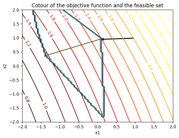
Now we will proceed with the implementation of this constrained optimization problem for some given values of $A$ and $b$. Empirically, we will observe that both approaches give us the same solution.
$$ A = \begin{bmatrix} 0.42653338 & 0.01419502 \\ 0.33599965 & 0.34548836 \\ 0.97202155 & 0.2533662 \\ 0.83768142 & 0.13944988 \\ 0.9881595 & 0.68442012 \end{bmatrix} b = \begin{bmatrix} 0.95011621 \\ 0.62676223 \\ 0.22844751 \\ 0.14841869 \\ 0.09432889 \end{bmatrix} \epsilon = 1 $$
Solving either directly primal and alternative dual ( we call this alternative because its not exactly dual because we added a new variable y) we get the same solution.
$$ x = \begin{bmatrix} -1.35816245 \\ 0.36198854\end{bmatrix} $$
| |
|---|
This problem is much simpler; the function $f(x)$ is linear or a relaxed version of logarithmic exponentiation. Directly solving constrained optimization problems is not always possible. Instead, we will work with an iterative approach called Projected Gradient Descent (PGD). The idea is that if the value of $x$ after every iteration is outside of the feasible space, we project it back to the feasible space.
Projected Gradient Descent
We will make a sketch of the termination criteria, We will write a proof for convergence which follows similar lines of proving convergence of gradient descent.
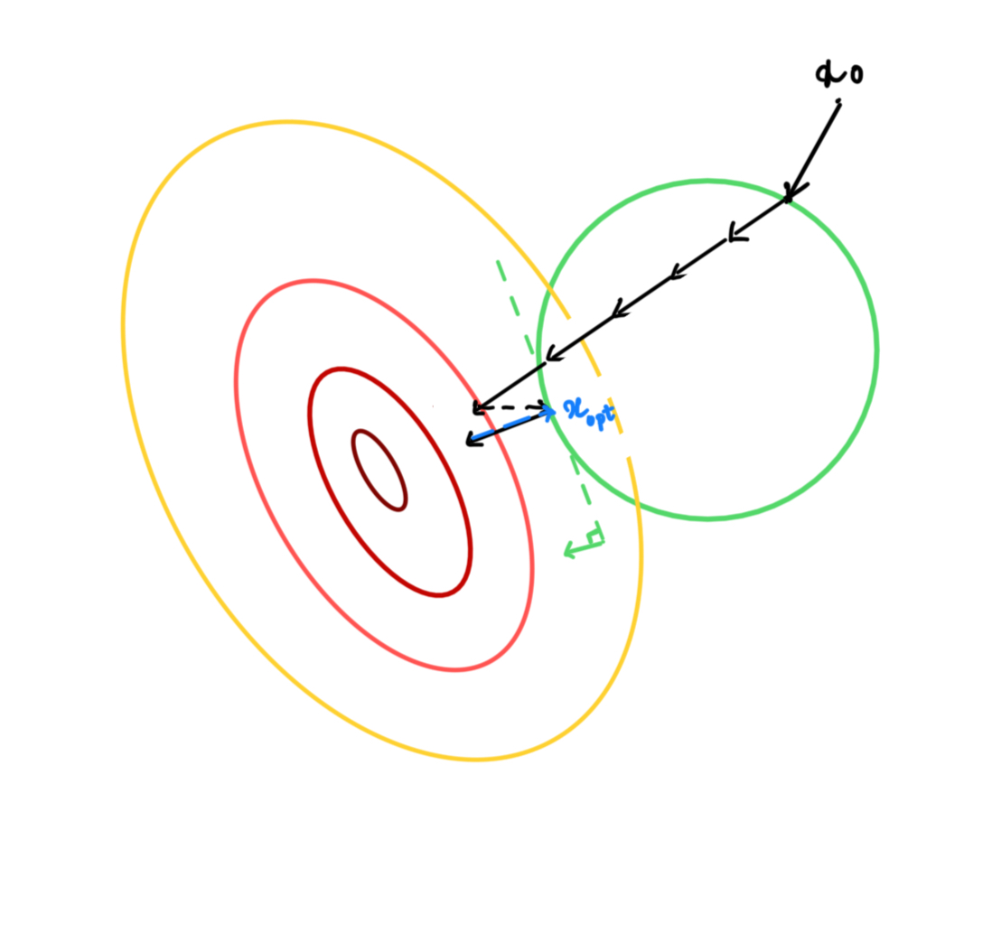
What is a projection operation
The projection involves solving a simpler optimization problem compared to the initial optimization, which is done as follows:
$$ \begin{align*} \min \quad & || x - \tilde{x} ||_2^2 \\ \textrm{s.t.} \quad & x \in \mathcal{C} \\ \textrm{where} \quad & \tilde{x} = x_t - \alpha \nabla f(x_t) \end{align*} $$
Proof of convergence
We will solve for the linear case and assume it extends to the non-linear case or leave the non-linear case for future consideration.
Assumptions:
- The function is differentiable.
- The function is Lipschitz smooth ($|| \nabla f(x_1) - \nabla f(x_2) ||_2 \le L || x_1 - x_2 ||_2$) ($H \le LI$).
- The function is convex (the derivative slope line is the lower bound everywhere).
- The constraint set is linear (can be extended to non-linear).
We start the procedure with $x$ in the set $\mathcal{C}$. If the initial $x$ is random, we can apply the projection to $x$ and choose a point in the convex set.
$$ \begin{aligned}\ f\left( x^{+ }\right) \leq f\left( x \right) + \nabla f\left( x\right) ^{T}\left( x^{+ } - x \right) +\frac{1}{2} (x - x^{+ })^TH (x - x^{+ }) \end{aligned} $$ Applying Lipschitz smoothness, $$ \begin{aligned}\ f\left( x^{+ }\right) \leq f\left( x \right) + \nabla f\left( x\right) ^{T}\left( x^{+ } - x \right) +\frac{L}{2} ||x - x^{+ }||_2^2 \end{aligned} $$ Let $P$ be the projection matrix onto the subspace. From linear algebra, we know that $P^2 = P$, $P^T = P$, and $Px = x$ for $x \in \mathcal{C}$. $P$ is positive semi-definite.
In gradient descent, we update the step as follows: $x^+ = x - \alpha \nabla f(x)$. In PGD, we add a new projection matrix, $P$, so the update step transforms to $x^+ = P(x - \alpha \nabla f(x))$ as per the property of the projection matrix. $x^+ = x - P \alpha \nabla f(x)$. As you can already see, this will stop when $\nabla f(x) \in \mathcal{N}(C)$.
Let’s substitute the step into the equation. $$ \begin{aligned}\ f\left( x^{+ }\right) \leq f\left( x \right) - \nabla f\left( x\right) ^{T} P\alpha \nabla f(x) +\frac{L}{2} || P\alpha \nabla f(x)||_2^2 \\ f\left( x^{+ }\right) \leq f\left( x \right) - \nabla f\left( x\right) ^{T} P\alpha \nabla f(x) + \alpha^2 \frac{L}{2} \nabla f\left( x\right) ^{T} P\nabla f(x) \\ f\left( x^{+ }\right) \leq f\left( x \right) - \alpha(1 - \frac{\alpha L}{2} ) \nabla f\left( x\right) ^{T} P\nabla f(x) \\ \end{aligned} $$
We know that P is positive semi definite, so $\nabla f\left( x\right) ^{T} P\nabla f(x) \ge 0$ and if $\alpha \le \frac{1}{L}$
$$ \begin{aligned}\ f\left( x^{+ }\right) \leq f\left( x \right) - \frac{\alpha}{2} \nabla f\left( x\right) ^{T} P\nabla f(x) \\ \tag{8} \end{aligned} $$ One thing to notice is function value is always decreasing.
Now, with the assumption of convexity, we will link the above equation to the optimum value. Let’s derive it from the convex assumption and substitute equation (8) into the convex assumptions. We know that the derivative is a lower bound everywhere for convex functions. We take the derivative at $x$ and interpolate it to $x^{\ast}$.
$$ \begin{aligned}\ f(x) &\leq f(x^{\ast}) + \nabla f\left( x\right) ^{T}(x - x^{\ast}) \\ f\left( x^{+ }\right) &\leq f(x^{\ast}) + \nabla f\left( x\right) ^{T}(x - x^{\ast}) - \frac{\alpha}{2} \nabla f\left( x\right) ^{T} P\nabla f(x) \\ f\left( x^{+ }\right) - f(x^{\ast}) &\leq \nabla f\left( x\right) ^{T}(x - x^{\ast}) - \frac{\alpha}{2} \nabla f\left( x\right) ^{T} P\nabla f(x) \\ \end{aligned} $$ We simplify the equation further, by adding and subtracting $\frac{1}{2\alpha} ||x-x^{\ast}||_2^2$ $$ \begin{aligned} f\left( x^{+ }\right) - f(x^{\ast}) &\leq \frac{1}{2\alpha}( ||x-x^{\ast}||_2^2 - || x - \alpha P\nabla f(x) - x^{\ast}||_2^2) \\ \sum_k f\left( x^{k }\right) - f(x^{\ast}) &\leq \frac{1}{2\alpha}||x^{0} - x^{\ast} ||_2^2 \\ f\left( x^{k }\right) - f(x^{\ast}) & \leq \frac{1}{2k\alpha}||x^{0} - x^{\ast} ||_2^2 \end{aligned} $$
This proves that the function is decreasing, and the error to the optimal value will get smaller and smaller with the number of steps. We can observe that this convergence behavior is the same as gradient descent.
Example problem
Sharing the results of the same problem mentioned above, this method provides us with the same solution as the earlier approaches but is more helpful for complex functions.
for epoch in range(100):
    x -= 0.01 * (A.T @ c)

    #solving primal projection operation
    new_x  = cp.Variable(x.shape)
    objective = cp.Minimize(cp.norm(new_x - x, 2)**2)
    constraints = [cp.norm_inf(A @ new_x + b) <= eps]
    prob = cp.Problem(objective, constraints)
    prob.solve()

    x = new_x.value
print(x)
Conclusion
We began with what seemed like a complex optimization problem. We employed lower bounds to transform it into a linear equation with non-linear constraints, which we further reduced to linear optimization. Then, we discussed the iterative method PGD and why it should be used for complex objective functions. In fact, we demonstrated that this iterative approach converges, similar to gradient descent, and showed that at convergence, the KKT conditions are satisfied. This proves that the solution is indeed optimal. As all the functions involved are convex, the solution is globally optimal.
Using optimiation for white-box adverserial attacks
Let’s design the adversarial attack. The attack will be clearer if we write the optimization equation, and we will use PGD to solve all the optimization equations.
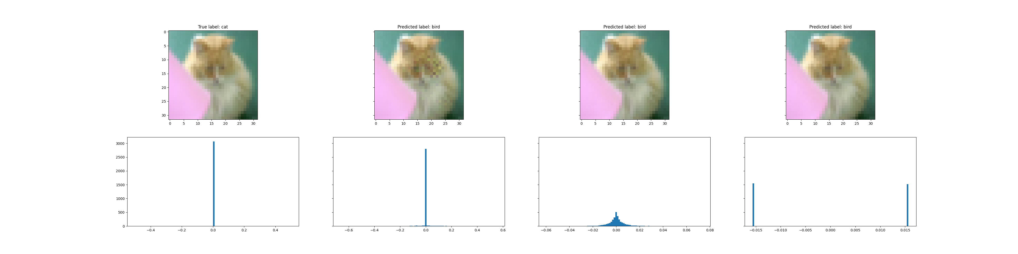
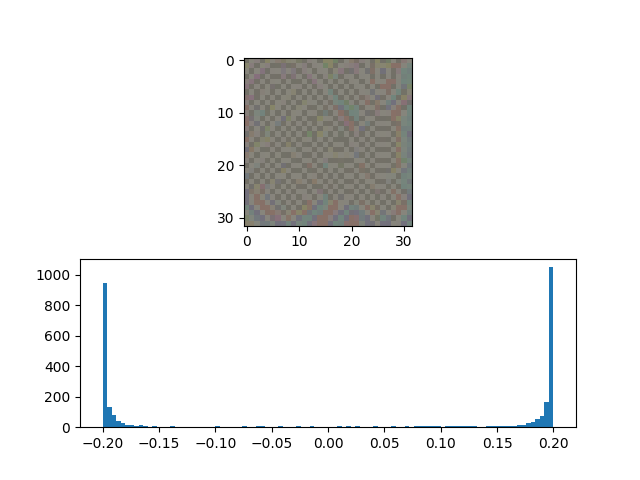
$$ \begin{align} \min_x & \quad f(x+\delta)_{y=t} - \max_{y \ne t} f(x) - \tau \\\ \textit{s.t} & \quad ||\delta||_p \le \epsilon \end{align} \tag{9} $$We can have $p = 1,2, \infty$. The properties of the attack and solution change accordingly to the choice of $p$. We will empirically explain how the histogram of $\delta$ looks like in each case of the $p$ value.
With PGD, we don’t have to solve the optimization. We only need to solve a simpler constrained optimization.
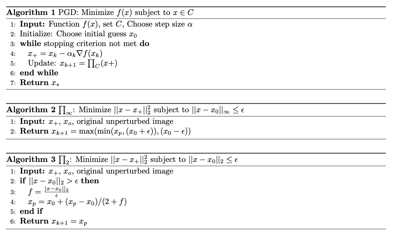
The stopping criteria is given by the perturbation when the attack is successful. Algorithms $2,\infity$ norm given in Algorithm 2 and 3 respectively can be solved by writing the dual and maximizing it. However, the 1-norm is not differentiable, so we don’t have a closed form solution. Instead, we can solve it with regularization and use the bisection method to find the right regularization for the given constraint.
In this post, we have chosen manually $\epsilon$, or the attack radius. However, we can formulate a complex optimization problem to determine the smallest $\epsilon$ possible for the attack to be successful. We will address ADMM and proximal gradient methods in another post.
Understanding Norm Minimization in Perturbed Spaces
This was directly adapted from Lecture 11, Convex Optimisation, S.Boyd
In the next section, instead of attacking one single image, we will design a template $\delta$ of a class, which when added to other images not belonging to the class, will cause them to be incorrectly classified.
Adverserial Templates and Attack Accuracy
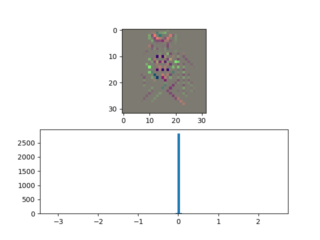 | 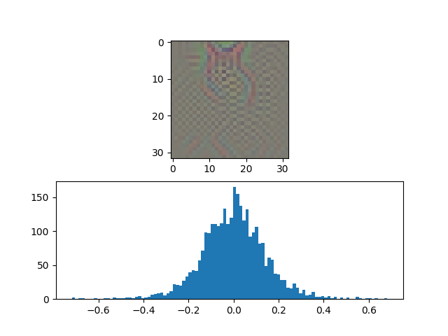 |  |
This Image presents the parameters and visual representations for an adversarial attack designed to fool all non-cat images into being classified as cat images. The top part represents the $\delta$ or the adversary that needs to be added, and the bottom plot represents the histogram of pixels.
| Parameter | Value |
|---|---|
| $\epsilon_1$ | 150 |
| $\epsilon_2$ | 8 |
| $\epsilon_{\infty}$ | 0.2 |
The values are chosen such that the test attack accuracy is close to 90%.
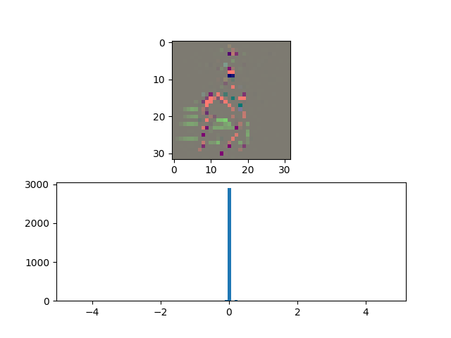 | 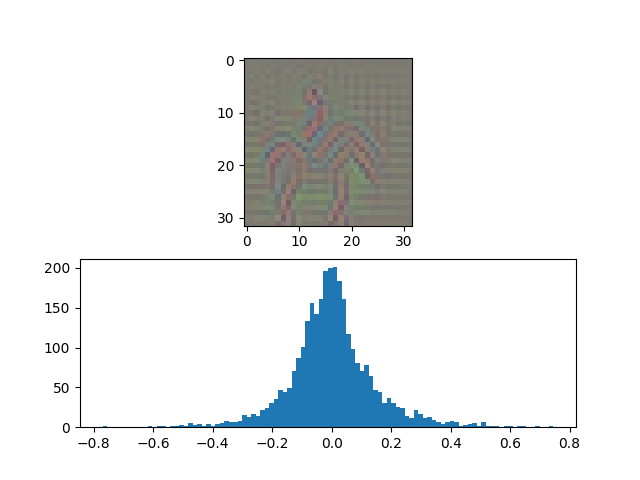 | 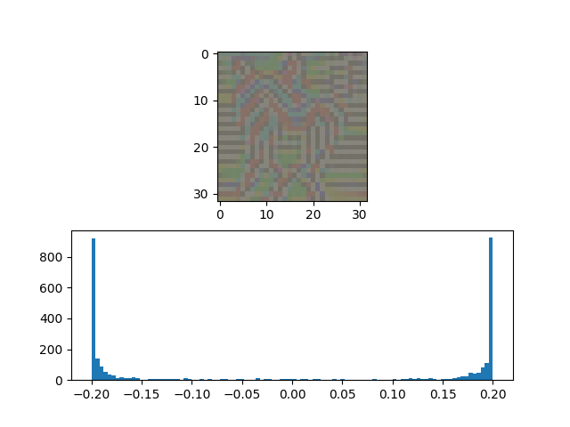 |
Image: Similar Results for Classifying Non-Horse Classes as Horse
References#
[1] S. Boyd and L. Vandenberghe, Convex Optimization. Cambridge University Press, 2004.
[2] S. Diamond and S. Boyd, CVXPY: A Python-embedded modeling language for convex optimization. Journal of Machine Learning Research, vol. 17, no. 83, pp. 1–5, 2016.
[3] Ryantibs, Convex Optimisation, Fall'13 Convergence of gradient descent
[4] Sachit, Code to the adove experiments